In 2015, DeepMind presented their Deep-Q-Learning algorithm. In this section we’ll explain their algorithm, a few variations that work better on Pong, and some complementary explanations.

Introduction: Q-Learning

The general idea should be familiar from the previous section. We want to estimate the \(Q^*\) function using an iterative algorithm performing the following update at every step:

Remember that we do not rely on a knowledge of the model now, so we simply cannot apply this update as-is as we don’t know \(\text{next}(s, a)\) and \(r(s, a)\). Instead, we interact with the game, while each step gives us a state, action, reward, and next state, which are being used to estimate \(\text{next}(s, a)\) and \(r(s, a)\) in the above equation. Once we have some estimated \(Q^{(i)}\) we can define the policy \(\pi_{i+1}\):

and play according to it. Each step of this play will give us a new tuple \((s, a, \text{next}(s,a), r(s, a))\). For every step, we can perform a single update of our estimated Q-Function.

It turns out that this algorithm doesn’t perform very well as is, because we might get stuck with a bad estimated \(Q\) that we can’t improve. So, instead of following \(\pi_ i\) from above, we follow \(\pi_i^{(\epsilon)}\):

with \(\epsilon\) being an exploration parameter, making us occasionally test new actions in case they’d turn out to be more profitable. For an MDP, this algorithm is guaranteed to converge to an optimal policy given enough time.

DeepMind’s Algorithm and Heuristics

So Q-Learning is a nice RL algorithm for a discrete state space. But Pong states are continuous, so we cannot apply it as is. Enter DeepMind and NN. As we saw in a previous section, we can adapt a discrete algorithm to the continuous case using NN. And essentially that was what DeepMind did in order to master the Atari 2600.

There were a few caveats. Apparently, when they implemented this algorithm they had “stability issues”: they managed to learn something but not consistently. So they added two heuristics that were meant to improve stability:

1. Replay memory: instead of updating their estimated Q-function using the sample alone, they store this sample (a 4-tuple \((s, a, \text{next}(s,a), r(s,a))\) ) in a DB, and randomly chose 32 entries from the DB, performing the Q-iteration update using those entries.
2. They use two different networks, \(Q\) and \(\hat{Q}\), the former is being used for deciding which action to take and is being updated after every step, while the latter is used to evaluate the Q-value. Every once in a while they set \(\hat{Q}=Q\).

Nothing was said about those heuristics in the original paper, except that they improve stability. Anyway, now we can present the full algorithm, as it appears in their paper:

1. Initialize replay memory \(D\) to capacity \(N\).
2. Initialize action-value function \(Q\) with random weights \(\theta\).
3. Initialize target action-value function \(\hat{Q}\) with weights \(\theta\).
4. For episode=1,...,M do
    1. For t = 1,...,T do
        1. Select \(a=\underset{a}{\text{argmax}}Q(s_{t},a) \) with probability \(1-\epsilon\), and uniformally otherwise.
        2. Perform \(a\) in the simulator, getting a new state \(s^\prime\) and reward \(r\).
        3. Record \((s, a, r, s^\prime)\) in \(D\).
        4. Sample mini-batch of \(\{(s_j, a_j, r_j, s_j^\prime)\}\) from \(D\).
        5. Set \(y_j=r_j + \gamma \max_{a^\prime} \hat{Q}(s_j^\prime, a^\prime)\).
        6. Preform a gradient step to minimize \((y_j - Q(s_j, a_j))^2\).
        7. Every \(C\) steps set \(\hat{Q} = Q\).

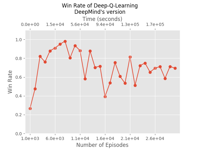
We implemented this algorithm exactly as is, and ran it for 8000 episodes, performing a total of 1385847 SGD steps (each on 32 samples). It took about 10 hours, and achieved 97% winning rate:

Simplified Algorithm

DeepMind algorithm works very well, but it seems overly complicated, and with some (yet) unjustified heuristics. Moreover, both DeepMind version and the classical Q-Learning don’t really follow the logic behind Q-iteration, which says to update the entire function at every update operation. Q-Learning only updates a single entry at every iteration and DeepMind’s version uses only 32 “examples” at every iteration. Finally, DeepMind’s algorithm is highly consecutive: we update the policy after each step, and certainly cannot run many episodes in parallel.

So, we decided to implement a simpler algorithm:

1. Play 1000 episodes using \(\epsilon\)-greedy policy based on current Q.
2. Use the sampled data to update the Q function estimation by performing a single Q-iteration on them.
3. Repeat.

We let it run for 26 generation, meaning 26000 episodes. It took about 15 minutes, and achieved 95% winning rate:

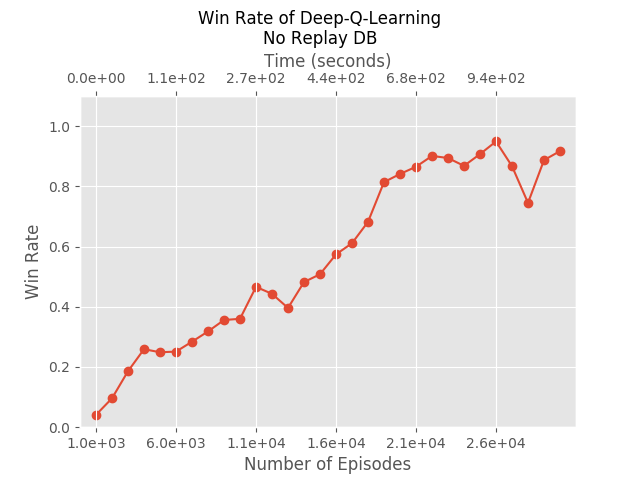
We can still see DeepMind’s “stability issues” - the policy doesn’t necessarily improve at every generation, even though overall it does get fairly good results. So we added a replay DB, just as DeepMind did. But, we also made it big enough to include all samples, and at every Q-iteration we use the entire DB. This gave us those results:

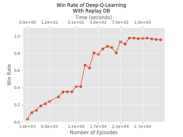
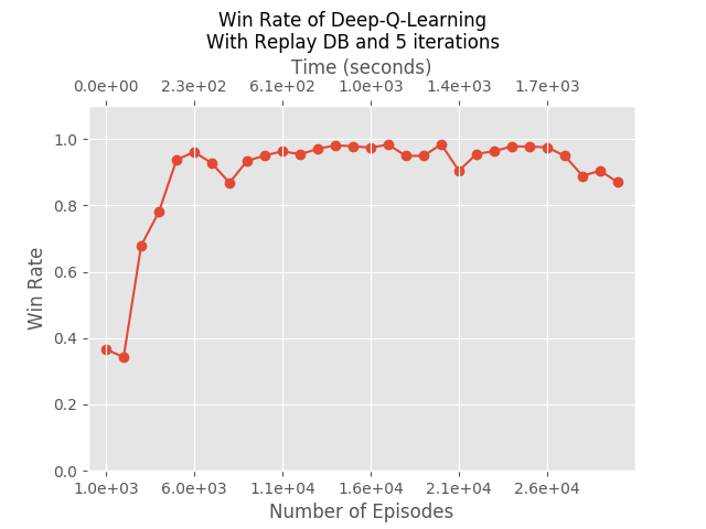
Indeed solving the stability issues. Finally, we asked why must we perform a single Q-iteration after every generation: hypothetically, we can perform many more. Those are the results if we perform 5 Q-iterations after every generation:

Analysis: Explaining DeepMind’s Heuristics

Why Replay?

The importance of the replay DB wasn’t clear to us at first, but after we saw its significance empirically, we understood that there is something deeper going on here. Moreover, reflecting on the replay DB effect allowed us to better understand what really happens in Q-Learning.

The real value of \(Q^*\) at a given state and action depends on its value on all states. That is, running many iterations of Q-iteration let “information” from every state to effect the final value at every other state. However, “closer” states affect more strongly. Specifically, in a single Q-iteration only values from neighboring states affect the state \(s\).

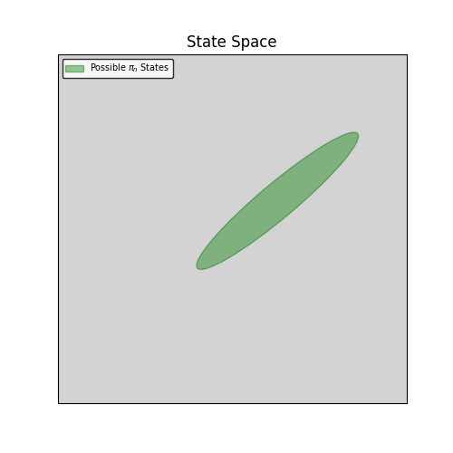
So, assume you start with a random policy \(\pi_0\). You get samples of the simulator at a few discrete points:

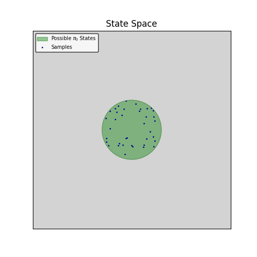
Now you run a single Q-iteration on those values. Because we’re using a NN, that have (some) generalization abilities, we get a slightly better approximation of the Q*-function at the surrounding area:

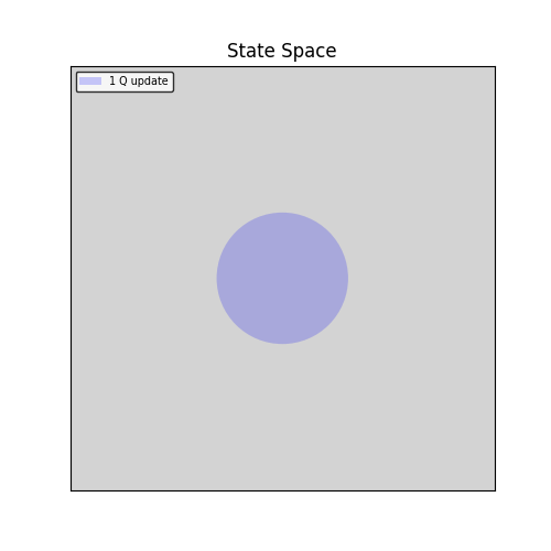
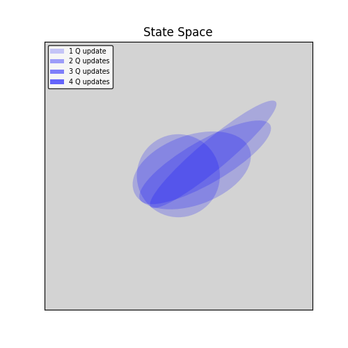
Now, you play according to a new policy \(\pi_1\), based on the updated \(Q\), and get new samples:

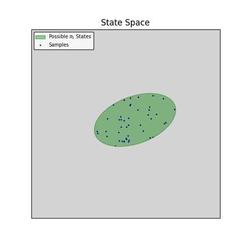
And again, performing a single Q-iteration gives you

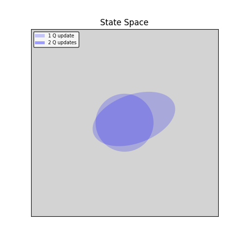
And so on. Finally you get a policy that’s very different from the original random one, perhaps something like that:

And this is how many times you updated the Q-value of the various states:

While with replay DB, we continually update the Q-function on all seen states, achieving something like that:

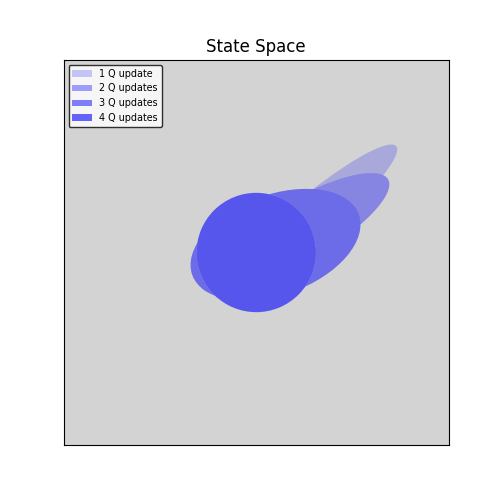
Now, it is a sad fact about training NN that if you train it with some distribution D, and than you train it again using a different distribution D’, you might get bad results on the original distribution D. Without a replay DB, we perform many Q-iterations on the value of the best policy. So eventually we will get good approximation of Q* on very few states, and very bad ones on the other states.

Remember the opening remark about the dependency of Q* on all states. The more states at which we approximate Q* the better approximation we will get. We cannot hope to know Q* at all states in this method within a reasonable amount of time - it would force us to sample all possible states. But it is enough to sample “around” the perfect policy, because far states effect very little on the Q* states that are really needed during a game according to \(\pi^*\).

So this is, we think, what the replay DB really does: it makes sure we approximate Q* at an environment of \(\pi^*\), giving us better approximations.

Why Target Network?

It’s not as easy to explain the role of the target network \(\hat{Q}\) in DeepMind’s original algorithm, because we don’t use it in the simplified version. But, in some sense we do something similar: we only run Q-iterations after collecting many samples. So we evaluate \(Q_i \) on all the states in the replay DB, and then we create \(Q_{i+1} \) based on those evaluation. This is similar in essence to DeepMind’s “target network” - using the same Q for evaluations. In what sense the two approaches are similar? Look at the following two algorithms:

1. Initialize replay memory \(D\) to capacity \(N\).
2. Initialize action-value function \(Q\) with random weights \(\theta\).
3. Initialize target action-value function \(\hat{Q}\) with weights \(\theta\).
4. For episode=1,...,M do
    1. For t = 1,...,T do
        1. Select \(a=\underset{a}{\text{argmax}}Q(s_{t},a) \) with probability \(1-\epsilon\), and uniformally otherwise.
        2. Perform \(a\) in the simulator, getting a new state \(s^\prime\) and reward \(r\).
        3. Record \((s, a, r, s^\prime)\) in \(D\).
        4. Sample mini-batch of \(\{(s_j, a_j, r_j, s_j^\prime)\}\) from \(D\).
        5. Set \(y_j=r_j + \gamma \max_{a^\prime} \hat{Q}(s_j^\prime, a^\prime)\).
        6. Preform a gradient step to minimize \((y_j - Q(s_j, a_j))^2\).
        7. Every \(C\) steps set \(\hat{Q} = Q\).

1. Initialize replay memory \(D\) to capacity \(N\).
2. Initialize action-value function \(Q\) with random weights \(\theta\).
3. Initialize target action-value function \(\hat{Q}\) with weights \(\theta\).
4. For episode=1,...,M do
    1. For t = 1,...,T do
        1. Select \(a=\underset{a}{\text{argmax}}\hat{Q}(s_{t},a) \) with probability \(1-\epsilon\), and uniformally otherwise.
        2. Perform \(a\) in the simulator, getting a new state \(s^\prime\) and reward \(r\).
        3. Record \((s, a, r, s^\prime)\) in \(D\).
        4. Sample mini-batch of \(\{(s_j, a_j, r_j, s_j^\prime)\}\) from \(D\).
        5. Set \(y_j=r_j + \gamma \max_{a^\prime} \hat{Q}(s_j^\prime, a^\prime)\).
        6. Preform a gradient step to minimize \((y_j - Q(s_j, a_j))^2\).
        7. Every \(C\) steps set \(\hat{Q} = Q\).

The only difference between the two is in line 4.1.1: whether to decide on an action using \(Q\) or \(\hat{Q}\). But, the second algorithm is equivalent to our “simplified algorithm” with replay DB: it’s true that it does a gradient step inside the inner loop, but there’s no reason for it - it doesn’t depend on the inner variables of the loop.

Why does it make sense? It improves the chances of succeeding in estimating \(Q_{i+1}\). We have much more samples. Updating Q based on a mini-batch of 32 entries essentially guarantees that occasionally we will fail: we are trying to learn a complicated function using a negligible amount of observations.

Double-Deep-Q-Learning

Let’s look again at the Q-iteration that stands at the base of Q-learning:

We can rephrase it as

Which might seem as a trivial manipulation, but actually it shows us that we use the \(Q\) network twice in every iteration: both to pick the best action (\(\text{argmax}\)) and to evaluate it. Without getting into details, it is a standard result in statistics that such estimates are often biased. It can be shown empirically that this is true in the Q-learning scenario as well, and that it might lead to suboptimal policies (or longer runtime until convergence). The Double-Q-Learning solution is to manage two functions, \(Q_ 1\) and \(Q_2\), and perform the updates:

In a 2016 paper, they showed how to change the original Deep-Q-Learning from above to match this insight, by changing the update formula accordingly, and it showed improved performances. While we can’t use this idea with our version of Deep-Q-Learning, we can add another network and perform the Double-Q-Learning literally, giving those results:

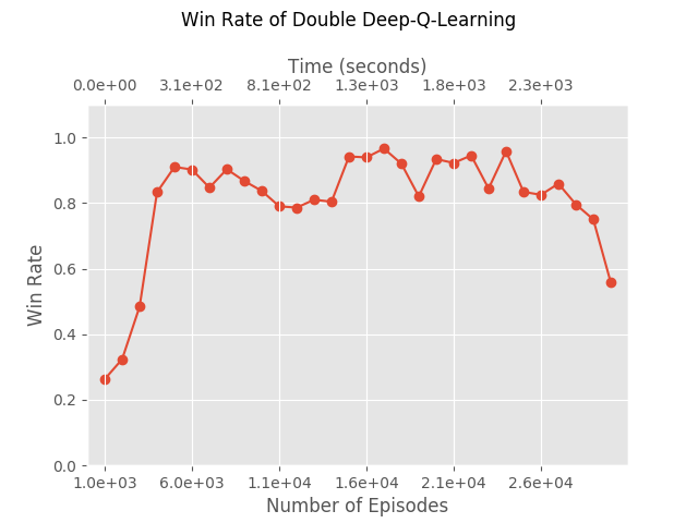
It is not impressive when compared to our “vanilla” version of Deep-Q-Learning, but it was worth trying because there are many reports that it gives better results. Perhaps one reason that we don’t see an improvement is that we use many episodes for each iteration (1000 episodes), so even if our estimates are biased, the bias is small. Had we tried to minimize the number of episode, it seems likely that at some point the Double-Deep-Q-Learning algorithm would have shown an improvement.

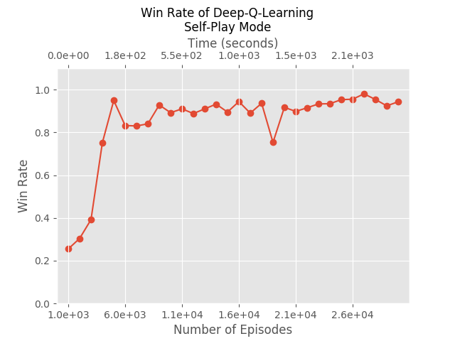
Self Play

Next Chapter

In Chapter 6: Learning While Playing Part 3, our final chapter, we describe some alternatives to Deep-Q-Learning, namely actor-critic methods: methods that are based on estimating \(Q_\pi\) for the current policy \(\pi\).