Actor-Critic: The Best of Both Worlds?

Let’s take another look at the Policy Gradient theorem:

$$\nabla_ \theta R(\pi_\theta) = \underset {\bar{s}, \bar{a} \sim \tau,\pi_\theta} {\mathbb{E}} \Bigg[ \left(\sum _{j=0}^T r(s _j, a _j)\right) ~ \sum _{i=0}^T \nabla _\theta \log(\pi _\theta (a _i | s _i)) \Bigg]$$

Which basically tells us we can get an unbiased estimator of the gradient of the objective by playing. But we can also get an unbiased estimator of the gradient by replacing \(\left(\sum _{j=0}^T r(s _j, a _j)\right) \) with many other functions - for example, any (positive) affine transformation of it will do. And, we can hope to be able to reduce the variance of the gradient by a wise selection of a function \(A(s,a)\) that would satisfy

$$\nabla_ \theta R(\pi_\theta) = \underset {\bar{s}, \bar{a} \sim \tau,\pi_\theta} {\mathbb{E}} \Bigg[ \sum _{i=0}^T A(s _i, a _i) \nabla _\theta \log(\pi _\theta (a _i | s _i)) \Bigg]$$

Intuitively, the Advantage Function is a good candidate for such a function. The advantage function attempts to capture the notion of “how good is the action a at state s compared to the other possible actions”, and its formal definition is

$$A_\pi(s, a) = Q_\pi(s, a) - V_\pi(s)$$

With the Q- and V- functions being the same ones we already met.

The Algorithm

1. Play 1000 episodes using \(\pi_{\theta_i}\).
2. Estimate \(Q_{\pi_{\theta_i}}\) by performing Q-Evaluation.
3. Create \(\pi_{\theta_{i+1}}\) by performing a single gradient step in the direction calculated by the formula above.
4. Repeat.

This kind of scheme is called “Actor-Critic” because we try to estimate how well our policy behaves (the “critic”, step 2), and then we use it to improve the policy (the “Actor”, step 3). Clearly, each iteration is much slower than vanilla PG, because we have to estimate the Q function at each step. But we can hope to get a much bigger improvement at every iteration. There are many other variations of “Actor-Critic” schemes, using different methods both for the “critic” part and the “actor-improvement” part.

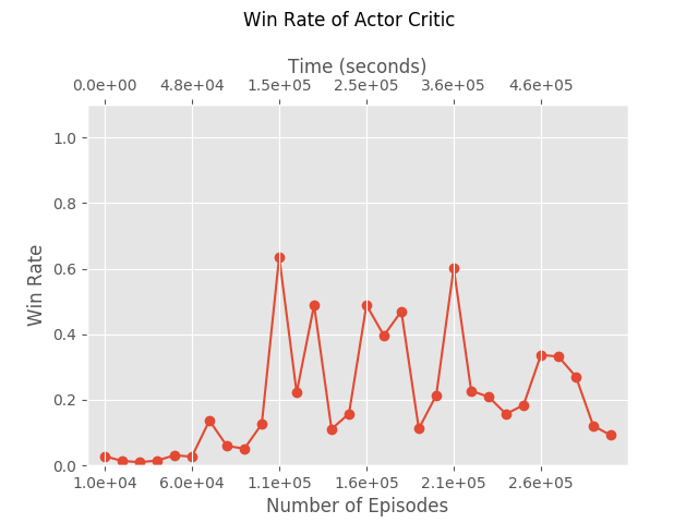
Results

We ran this version of AC, estimating the Q function and the gradient using 1000 episodes, for 470 generations, and got to 60% win rate.

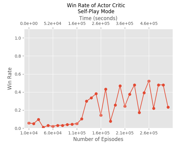
Self Play

Success Learning with a Critic

Success Learning is essentially a variation of PolicyGradient, where instead of learning from both successful and failed episodes, we learn only from successful ones, and we do multiple SGD steps with every iteration. In Actor-Critic methods we try to improve the learning by giving proper weights to the different moves. Just as we used a critic to improve PolicyGradient, we can do it with Success Learning.

The Algorithm

1. Play 1000 episodes using \(\pi_{\theta_i}\).
2. Estimate \(Q_{\pi_{\theta_i}}\) by performing Q-Evaluation.
3. Throw away all steps where the advantage of the step is negative.
4. Create \(\pi_{\theta_{i+1}}\) by Imitating the remaining steps.
5. Repeat.

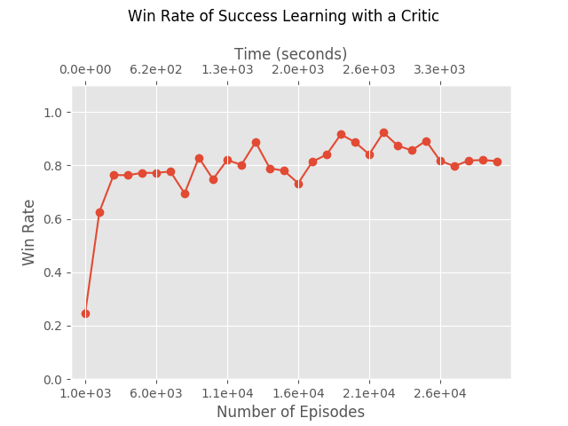
Results

This algorithm is actually quite impressive. While Success Learning is fast and stable, it doesn’t really compete with Deep-Q-Learning in how efficient it is in playing few episodes. This variation, adding a critic to SuccessLearning, fixes it. This algorithm is both fast and uses the least number of episodes of all the algorithms we presented so far.

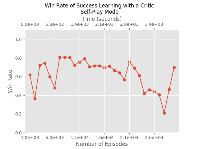
Self Play

Deep-P-Learning: All Together Now

This is the last algorithm we will present here, and it incorporates most of the ideas that appeared above, in one way or another. The name “Deep-P-Learning” doesn’t appear in the literature, but similar algorithms do appear. It is closest in spirit to the famous SARSA algorithm. We decided to give it this name because of its conceptual similarity to Deep-Q-Learning.

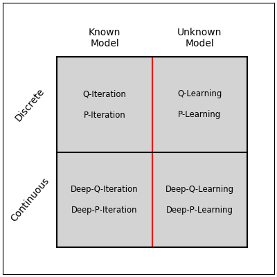
Deep-Q-Learning was created from the Q-Learning algorithm, which in turn was created from Q-Iteration. That is, Deep-Q-Learning is a function approximation, model free version of Q-Iteration. Similarly, Deep-P-Learning is a function-approximation, model-free version of P-Iteration.

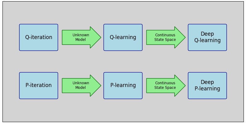
P-Iteration is known to achieve good policies in a small number of iterations, but each iteration is much more computationally demanding than Q-Iteration. However, in our case minimizing the number of iterations (=generations) is a legitimate objective on its own, and so Deep-P-Learning might prove to be useful in some situations.

The Algorithm

1. Start with a random \(\pi_{\theta_0}\).
2. Play 1000 episodes using \(\pi_{\theta_i}\).
3. Estimate \(Q_{\pi_{\theta_i}}\) by performing Q-Evaluation.
4. Define \(\pi_{\theta_{i+1}}\) such that \(\pi_{\theta_{i+1}}(s) = \underset{a}{\text{argmax}} Q_{\pi_{\theta_i}}(s, a)\).
5. Repeat.

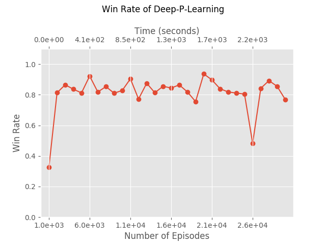
Results

It’s surprising how well this algorithm performs, occasionally achieving 50% winning rate within a single generation. That is, we play 1000 episode using a random policy, and immediately learn from them how to win in 50% of the games. This does not happen consistently, but it does consistently achieve win rate of above 20% in a single generation.

The Differences from Deep-Q-Learning

Here’s a possible explanation why this algorithm performs better than Deep-Q-Learning. Deep-Q-Learning attempts to evaluate Q* directly, and there is simply no way to do that using only random samples. It must update its Q function approximation gradually, performing new episodes according to the new policy at all times, because the value of Q* really depends on many not-yet-seen states. But it is possible to estimate \(Q_\pi \) by observing only episodes played by \(\pi \). It’s true that we have no reason to expect to reach Q* after a single iteration. Our claim is that Deep-P-Learning successfully mimics the classic P-Iteration algorithm, and therefore requires very few iterations, while Deep-Q-Learning is much worse then Q-Iteration.

Is it the true reason that this algorithm performs so well? The honest answer is that we don’t know. Perhaps it’s just luck. We didn’t optimize over any of the hyper-parameters, and it might be that our arbitrary choices happened to be well suited to this algorithm. A wise choice of hyper-parameters may bring the other algorithms to similar performances.

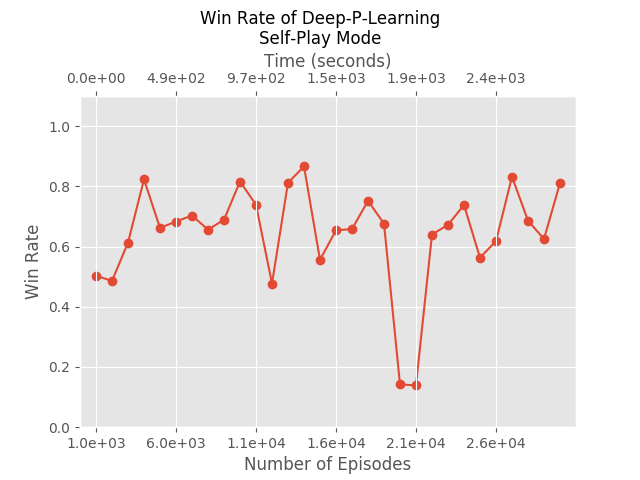
Self Play

Next Chapter

Well, this is the last chpater, so there is no “next chapter”. But we provide some References for further reading, if you’re interested.