Perhaps the most impressive recent success of RL is DeepMind’s AlphaGo, an algorithm that managed to achieve superhuman capabilities in the classic game of Go. Their first algorithm, called simply AlphaGo, used many of the ideas we already saw, and many others as well. Their second algorithm, AlphaGo-Zero (AGZ), achieved better results, and is more interesting for our purposes, as it presents a whole new RL algorithm. AGZ is also different from AlphaGo in that it’s not based on a sample of human expert games as a part of its training, while AlphaGo did.

AlphaGo (both variants) was designed to solve Pong-like games: we are looking for a policy that can defeat any rival policy, and not Snake-like games where we are looking for an optimal policy in a constant environment. However, it can be understood as the combination of two algorithms: one that solves Snake-like games, and than a transformation that makes it more robust against different rivals. Both parts are necessary for the success of AlphaGo, but each is interesting on its own. We will start with the first one: an algorithm for finding an optimal policy for a known MDP, an alternative to V/Q/P Iteration.

AlphaGo-Zero

The AlphaGo-Zero Hypothesis

Recap: MCTS is an algorithm, that given some policy \(\pi\), returns a non-explicit policy \(\text{M}(\pi)\). “Non-explicit” here means that you only get \(\text{M}(\pi)\) algorithmically: you can calculate \(\text{M}(\pi)(s)\) for a given \(s\), but you must do it separately for every \(s\).

Now we can informally phrase AGZ underlying assumption:

Even with a small number of simulations, \(\text{M}(\pi)\) is always significantly better than \(\pi\).

Which is not unreasonable: MCTS performs very well in many situations, using a constant number of simulations.

Algorithm Description

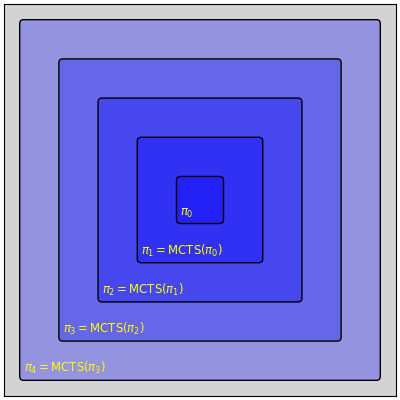
The basic idea of AGZ is that we want to use \(\text{M}(\text{M}(…\text{M}(\text{M}(\pi_ 0))…))\) for some arbitrary \(\pi_0\). According to the AGZ hypothesis, \(\text{M}(\pi)\) is better than \(\pi\), \(\text{M}(\text{M}(\pi))\) is better than \(\text{M}(\pi)\) and so on. It means that many applications of \(\text{M}(\cdot)\) should give us a very strong policy. It is theoretically possible that \(M(\pi)\) is always better than \(\pi\), but that \(\text{M}^n(\pi)\) is still bounded and achieves suboptimal policy, so this is the formal meaning of “significantly” from before. So the (semi-)formal phrasing of the AGZ hypothesis is:

For every \(\pi_ 0\), \(\text{M}^n(\pi_0)\) converges quickly to an optimal policy.

This is a very interesting observation on its own, but its not an algorithm yet. Calculating \(\text{M}^n(\pi_0)(s)\) is computationally intractable. Remember that \(\text{M}(\pi)\) is given in a non-explicit way. A single evaluation of \(\text{M}(\pi)(s)\) requires performing many simulations - that is, many calls to \(\pi\). So a single evaluation of \(\text{M}(\text{M}(\pi))(s)\) would require many evaluations of \(\text{M}(\pi)\), each of which would require many calls to \(\pi\), and so on.

The next idea should be already familiar: starting with some \(\pi_ 0\), we will create an explicit policy \(\pi_ 1\) that approximates \(\text{M}(\pi_ 0)\). Then we can repeat the process: \(\pi_ 2\) will approximate \(\text{M}(\pi_1)\) and so on.

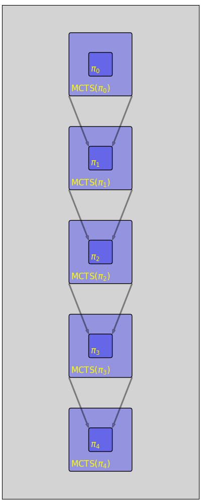
How can we find an explicit policy \(\pi_ {i+1}\) that approximates \(\pi_ i\)? Imitation. We can think about \(\text{M}(\pi_i)\) as an expert, let it play many episodes, and then Imitate it using a NN.

Learning the Value Function

So far we assumed we are using MCTS without a value function, and that we’re running every simulation till its end. Presumably this should work, but AGZ does use a value function, perhaps because it makes the algorithm more efficient. How can we estimate \(V_ {\text{M}(\pi)}\)? We can play full games according to \(\text{M}(\pi)\), and then approximate \(V_ {\text{M}(\pi)}\) directly: for every state s we saw in those games, we get a sample of \(V_{\text{M}(\pi)}(s)\).

The Algorithm

Start with some \(\pi_ 0\) and \(V_ 0\), and then:

Play many episodes using \(\text{M}(\pi_i)\).
Create \(\pi_ {i+1}\) by imitating \(\text{M}(\pi_i)\) on those games.
Create \(V_{i+1}\) by approximating \(V_{\text{M}(\pi_i)}\) based on those games.
Repeat.

Neat, isn’t it?

Addressing the Two Player Setting: Self-Play

So far we have described a method for finding an optimal policy for an MDP, much like V-Iteration. But AGZ is about more than that: it solves Go, where the rival policy is not known beforehand. But, remember that if we fix a rival policy, the game becomes an MDP. So we can fix the rival policy to be the same as the current policy: both sides are using the same policy. The algorithm then becomes:

Play many episodes using \(\text{M}(\pi_ i)\) against \(\text{M}(\pi_i)\).
Create \(\pi_ {i+1}\) by imitating \(\text{M}(\pi_i)\) on those games.
Create \(V_ {i+1}\) by approximating \(V_ {\text{M}(\pi_i)}\) based on those games.
Repeat.

The rationale behind this is that we expect the policy to gradually improve. \(\text{M}(\pi_ 1)\) is trained to defeat \(\text{M}(\pi_ 0)\). \(\text{M}(\pi_ 2)\) is trained to defeat \(\text{M}(\pi_1)\) and so on. If “\(a\) defeats \(b\)” is transitive, the last policy should defeat all the previous ones, and hopefully it means that it’s good enough to beat other policies as well.

AlphaPong-Zero

Now that we (the human race) managed to find an algorithm that masters the game of Go, we can finally address the real issue: mastering Pong. In other words, using AGZ to solve Pong is the RL equivalent of using nuclear weapons to clean your home from dust. While technically it should work, it’s still the wrong solution. However, we hoped to get some insight about AGZ itself. So we wrote our own implementation of AGZ for Pong, or AlphaPong-Zero (APZ). Our implementation is a pure python implementation (using tensorflow for NN), so it’s very slow. While most of the other algorithms in this review take anything from few minutes to few hours to run, APZ needs a few days.

Results

It is unclear how should we test APZ. AGZ ends its training phase with some policy \(\pi_ n\), and plays its games according to \(\text{M}(\pi_ n)\), using a time-conscience version of MCTS (doing as many simulations as the time allows). So, should we test the final policy APZ got (\(\pi_ n\)), or \(\text{M}(\pi_ n)\)? On the one hand, using \(\text{M}(\pi_ n)\) is more similar to AGZ. On the other hand, it is unfair when compared to other algorithms: they had to find an explicit policy, but \(\text{M}(\pi_ n)\) is an implicit policy.

In theory, there shouldn’t be a great difference between the two. If the imitation step works perfectly, then \(\pi_ n = \text{M}(\pi_ {n-1})\). So we can just train APZ for another iteration, and use the new policy, instead of using \(\text{M}(\pi_ n)\). But unfortunately, this is not the case.

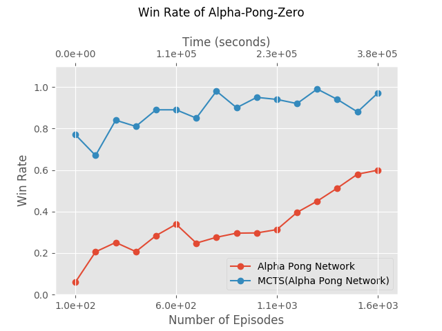
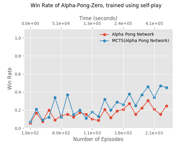
Those two graphs were supposed to be the same with a shift of 1, and they’re clearly not. It tells us that the imitation worked rather poorly. But, is does work, to some extent: otherwise we wouldn’t see any improvement at all (on both graphs).

It is our belief that it happened mainly because we used too few episodes in each iteration: we used 100 episodes, and Imitation simply cannot succeed with so few episodes. We would let it run with 1000 episodes per iteration, but it takes about 8 hours for every iteration now, and doing 1000 iteration would require 80 hours.

APZ without MCTS.

APZ with MCTS.

Self Play

As we said, AGZ was specifically designed to work in a Pong-like scenarios. Using it in a Snake-like scenario, as we did in the previous section, is somewhat bizarre. However, for reasons we don’t fully understand, it doesn’t work as well as we expected. It might be because we didn’t use enough iterations, or perhaps it is because of the self-play scheme we used.

APZ that was trained in self-play, without MCTS.

APZ that was trained in self-play, with MCTS.

Win rate of both version of APZ, trained in self-play mode.

Thoughts

AGZ works by playing according to \(\text{M}(\pi_ i)\) and imitating it. But technically, we can run \(\text{M}(\pi_ i)\) on any state we wish, not necessarily as a part of an episode. And, if we learned one thing from the Imitation section, is that it is much better to run your expert on random states and not on full episodes. AGZ doesn’t do it for a good reason: applying \(\text{M}(\pi_ i)\) to a truly random Go board is probably useless, because truly random Go boards tell us very little about possible Go boards. By letting \(\text{M}(\pi_i)\) play only full episodes, it ensures we at least sample some important states. On the other hand, it makes the imitation much more difficult. There might be a compromise between the two approaches: using both full episodes and somewhat randomized states, for example by using a replay DB. This will enlarge the number of states over which we apply the Imitation.

There’s a deeper issue here. In the current implementation of AGZ, \(\pi_ {i+1}\) approximates \(\text{M}(\pi_ i)\) only in states that can be reached by playing according to \(\text{M}(\pi_ i)\). But, when it uses \(\pi_ {i+1}\) it evaluates it on many more states - specifically, on states that were reached by playing according to \(\text{M}(\pi_ {i+1})\). So in essence, we have very little reason to believe that \(\pi_ {i+1}\) approximates \(\text{M}(\pi_i)\) well on the states that actually interest us.

This issue can probably be solved by using some sort of iterative method: approximating \(\pi_{i+1}\) many times, each time on a new set of states. This would be computationally expensive, and not necessarily more useful than simply running more iterations of AGZ, but it will be more justified.

Next Chapter

In Chapter 4: Learning While Playing Part 1 we move on to a different scenario - we attempt to learn a policy when all we can do is interact with the environment, and we have no knowledge of the rules. We start with a short description of the problem, and then decribe the Policy Gradient algorithm and a simple variation of it.