Assume you want to learn how to play a game by watching an expert playing it. You have no idea what the rules are, and can’t interact with the game in any way, so your only option is to try and do whatever the expert does. If this seems absurd to you, just watch some youtube videos of experts playing video games.

This is the idea behind Imitation. If you have access to the games of an expert, you first create a sample of \(\{(\text{state}_i, \text{expert action}_i)\}\), and then use any Supervised Learning (SL) algorithm you like so as to learn a policy that mimics the expert. Because SL algorithms perform very well, it is supposed to work great. Obviously, imitation has a serious limitation: you cannot expect to become better than the expert — if you are aiming for super-human performance, you cannot get there by imitating humans.

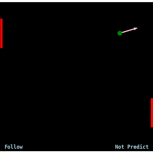
In this part we only deal with the snake-like scenario: the left paddle is assumed to be fixed to “Follow”, and we try to learn a policy for the right paddle, that imitates “Predict”.

First Attempts

We collected 200000 observations from “Follow” vs. “Predict” games, and trained our NN to match the actions of “Predict”. As it’s a simple classification problem, we expected it to succeed, and indeed got 97% test accuracy after 150 epochs. With the intent to move on to more interesting algorithms, we tested it by letting the resulting NN play against “Follow”. It turned out it lost 99% of the games, which was more than a little disappointing. Here’s how it looks like:

This is somewhat surprising. Despite having 97% accuracy on the test set (so it can’t be explained by overfitting), it mimics the “Predict” policy very poorly. At first we thought it might be because “Predict” is very sensitive to noise, so that even few mistakes can cause a drastic change in overall performance. We ruled out this hypothesis by adding random noise to the “Predict” policy, and observing that it still wins consistently (even with 20% noisy actions). It looks like this:

Before we tried to explain this, we made another test. The “Predict” policy is a composition of two functions: the first takes the current position and velocity of the ball and calculates where it will hit the end of the table. The second takes the output of the first and the location of the paddle, and decides whether to go up, down, or stay. So we tried to mimic only the first function and manually apply the second. This improved things a bit (we got 34% winning rate), but is still disappointing:

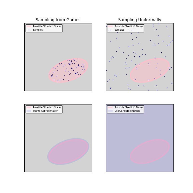
Anyway, at this point we became really annoyed. As a final test, we created a new sample of 200000 observations, but this time not by simply watching “Follow”/“Predict” games, but by setting the game state to random values and seeing how “Predict” behaves. Essentially, we collected samples of “Predict” over a uniform distribution — you can think of it as throwing the ball randomly into the table and watching how our expert responds. The performance of the NN on the test set was similar to before, but the winning rate was dramatically better (94%):

Note that this algorithm requires a more intimate knowledge of the expert relatively to the original Imitation scenario: we don’t only assume we can observe it while it plays, but that we can actively interfere with it.

What Happened: Distribution Drift

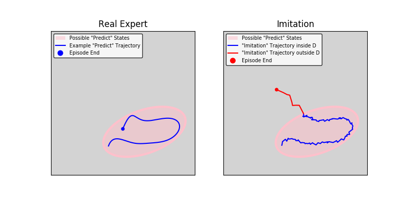
Assume we let “Predict” play against “Follow” for a long time, and that we sample the state and its action at a random point. Call the distribution over the state-space that we get in this way \(G\). Our sample for the first two tests came from this distribution (admittedly not in an i.i.d. fashion, because we used full episodes). So, our NN got high accuracy over this distribution. But, when playing with the learnt policy, because it didn’t learn perfectly, the state distribution is now different: call it \(G^\prime\). And, the NN apparently approximate “Predict” over \(G^\prime\) very poorly. It is actually unfair to expect it to be accurate over a different distribution than the one it was trained upon.

Put differently, when we let the NN play, it did alright for a few steps, but at some point it made a mistake or two, which put it in a never-before seen situation. Because “Predict” is such a good policy, there are states that simply cannot happen with it:

And once the NN arrived to such a state, it basically behaved randomly, meaning it is not surprising it lost quickly. The following illustration demonstrate it:

Sampling uniformally avoids this problem, because we have reasonable approximations of “Predict” even for impossible situations:

Finally, Success

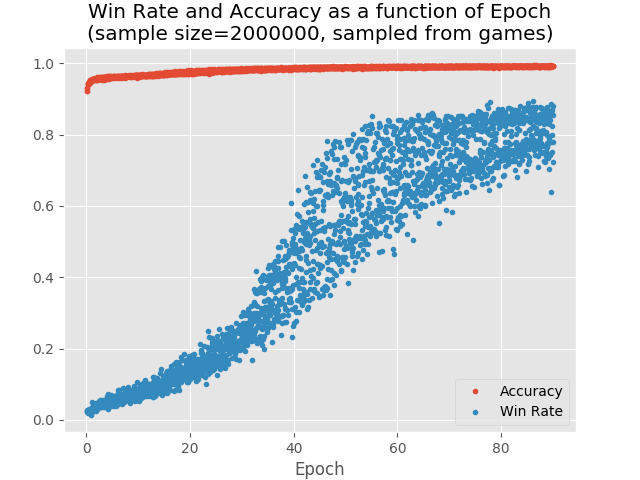
In order to test this explanation, we wanted to test and see if indeed the amount of distribution drift is inversely correlated to the NN accuracy. We considered various ways to improve the accuracy, but the simplest one was to use many more observations and running the training for many more epochs. So, we used 2000000 observations and 900 epochs, and finally got 85% winning rate (with 99% accuracy).

This graph shows the winning rate as a function of the prediction accuracy:

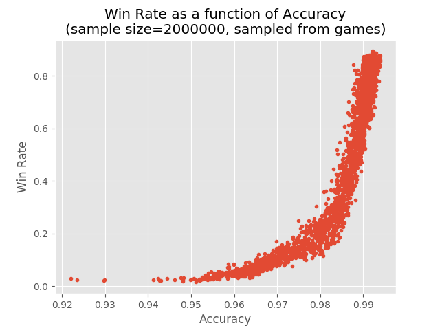
Pay attention to the values on the accuracy axis: even a 0.2 percentage point improvement in accuracy can create a 70 percentage points improvement in winning rate.

This is a graph of accuracy and win rate as a function of the number of epochs:

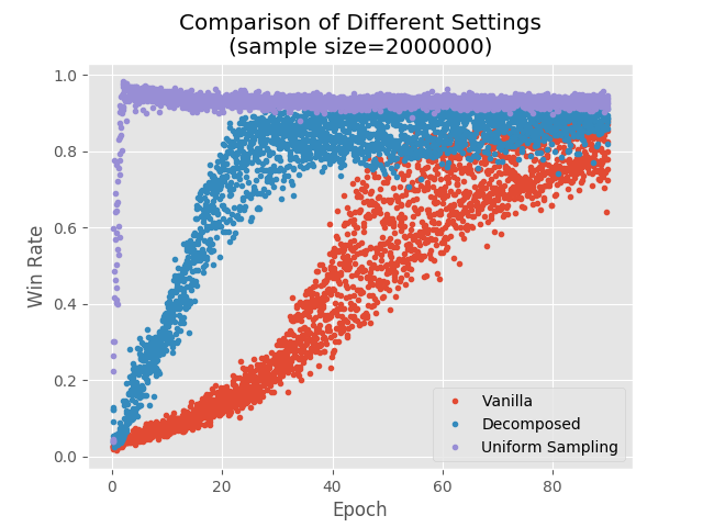
And here’s a comparison between the three different settings we discussed:

Conclusions

This case serves as a great demonstration of the difficulty of RL problems. Even in the supposedly easy Imitation scenario, when we reduced the RL problem into a SL problem, it still turned out to be much harder than expected. It also shows that distribution drift is a real problem: if you have a policy that performs relatively well, it doesn’t mean you will be able to imitate it and achieve good results without ridiculous amounts of data.

Next Chapter

As we saw, there are many limitations to this approach, not the least of which is that hardly ever we really do have an expert. In Chapter 2: When You Know the Model we don’t assume that, but we do make a different assumption: that we have perfect knowledge of the rules of the game, and only need to find the best policy for those rules.